Finite element method getting started examples

Finite element method getting started examples#

The following page is intended as an example of both the

interaction between numpy and ngsolve in teaching, as well as
for ngsolve in a Markdown file.

One-dimensional case#

As an introduction to the finite element method, let us consider the scalar boundary value problem

(1)#\[\begin{split}\begin{split} -u''(x) & = f(x)\quad\forall\ x\in (0,1)\\ u(0) & = u(1) = 0, \end{split}\end{split}\]

with \(f(x) = 1\).

We can easily obtain the analytical solution in this case. By integrating the right-hand side twice, we obtain a 2nd order polynomial

\[u(x) = \frac{1}{2} x^2 + C_1 x + C_2.\]

By inserting the boundary conditions, the analytical solution follows

\[u(x) = -\frac{1}{2} x (x-1).\]

def uanalytic(x):
    return -0.5*x*(x-1)

For the numerical solution, we multiply the differential equation with an arbitrary test function \(v(x)\in C_0^\infty(0,1)\) and integrate over the interval \((0,1)\)

\[-\int_0^1 u''(x) v(x)\,dx = \int_0^1 f(x) v(x)\,dx \quad\forall\ v\in C_0^\infty(0,1).\]

Using partial integration, we obtain the weak equation

\[\int_0^1 u'(x) v'(x)\,dx - \underbrace{\big[u'(x) v(x)\big]_0^1}_{=0\, \text{since}\, v(0)=v(1)=0} = \int_0^1 f(x) v(x)\,dx \quad\forall\ v\in C_0^\infty(0,1).\]

The weak problem is given by: Find \(u(x)\) such that \(u(0)=u(1)=0\) and

(2)#\[\int_0^1 u'(x) v'(x)\,dx = \int_0^1 f(x) v(x)\,dx \quad\forall\ v\in C_0^\infty(0,1).\]

To fulfill the equation, the solution \(u\) does not necessarily have to be a twice continuously differentiable function. Instead, \(u\) and \(v\) are each differentiated once. It is sufficient to use the functions from the Sobolev space \(H_0^1(0,1)\). The right-hand side also no longer has to be continuous. It is sufficient if the function \(f\) is square integrable, hence \(f\in L_2(0,1)\). From the problem (2) we obtain solutions which do not always necessarily have to be solutions of the strong equation (1).

Let us discretize the interval \((0,1)\) into subintervals \((x_{i-1},x_i)\) for \(i=1,\ldots, n\). On this decomposition we define the basis functions

\[\begin{split}\varphi_i(x) = \begin{cases} \frac{x-x_{i-1}}{x_i-x_{i-1}}\quad \text{for}\ x \in (x_{i-1},x_i)\\ \frac{x_{i+1}-x}{x_{i+1}-x_{i}}\quad \text{for}\ x \in (x_{i},x_{i+1})\\ 0\quad \text{else,}\end{cases}\end{split}\]

with which we approximate the Sobolev space \(H_0^1(0,1)\).

Numpy solution#

In the figure Fig. 2, the interval is divided into 5 subintervals. Accordingly, we have 5 +1 basis functions. Apart from the first and last basis function, the support extends over two subintervals in each case. The basis functions are exactly one in one node \(x_i\), in all others the function value is 0.

_images/adaa2123221e41fe52b049b99ba467876eb412c30094e64a23d7f7a3bc47632b.png — Fig. 2 FEM 1d first order basis functions#

For the weak equation (2) we obtain the finite dimensional problem: Find

\[u_h(x) = \sum_{i=0}^n u_i \, \varphi_i(x)\]

such, that \(u(0) = u(1) = 0\) and

(3)#\[\int_0^1 u_h'(x) \varphi_j'(x)\,dx = \int_0^1 f(x) \varphi_j(x)\,dx \quad\forall\ j = 1, \ldots, n-1.\]

Applying \(u_h\) into (3) leads to the system of equation

(4)#\[\sum_{i=0}^n u_i\ \int_0^1 \varphi_i'(x) \varphi_j'(x)\,dx = \int_0^1 f(x) \varphi_j(x)\,dx \quad\forall\ j = 1, \ldots, n-1.\]

We define the matrix \(A\) and the vector \(b\)

(5)#\[\begin{split}\begin{split} A_{j,i} & = \int_0^1 \varphi_i'(x) \varphi_j'(x)\,dx\\ b_j & = \int_0^1 f(x) \varphi_j(x)\,dx \end{split}\end{split}\]

and obtain the (reduced) linear system of equations for the coefficients \(u_1, \ldots, u_{n-1}\)

(6)#\[\sum_{i=1}^{n-1} A_{j,i} u_i = b_j \quad \forall\ j=1, \ldots, n-1.\]

or in compact form

\[A\cdot \vec{u} = \vec{b}\]

with \(\vec{u} = (u_1, \ldots, u_{n-1})^T\) and \(\vec{b} = (b_1, \ldots, b_{n-1})^T\). Due to the Dirichlet boundary conditions we have \(u_0 = u_n = 0\).

Assuming an equidistant decomposition as in the example above Fig. 2, we get

\[\begin{split}\varphi_i'(x) = \begin{cases} 1/h\quad \text{für}\ x\in (x_{i-1},x_i)\\ -1/h\quad \text{für}\ x\in (x_{i},x_{i+1})\\ 0 \quad \text{sonst.}\end{cases}\end{split}\]

_images/621e189570b671b5436c72c846baefc6233cdb93db2436319760a736b02e0d0c.png — Fig. 3 Derivative 1d first order FEM basis functions#

For the specific example, we obtain the matrix \(A\):

array([[ 5., -5.,  0.,  0.,  0.,  0.],
       [-5., 10., -5.,  0.,  0.,  0.],
       [ 0., -5., 10., -5.,  0.,  0.],
       [ 0.,  0., -5., 10., -5.,  0.],
       [ 0.,  0.,  0., -5., 10., -5.],
       [ 0.,  0.,  0.,  0., -5.,  5.]])

Exercise

Compute the coefficients by hand.

Analog follows for the right-hand side with concrete function \(f(x) = 1\):

array([0.1, 0.2, 0.2, 0.2, 0.2, 0.1])

The FEM solution \(u(x)\) is therefore given by the solution of the system of equations (6) with the calculated system matrix and right hand side vector. Since the boundary values are given, only the inner degrees of freedom are used. The result is

u = np.zeros_like(xi)

# We will deal with the choice of linear equation solvers later:
u[1:-1] = np.linalg.solve(A[1:-1,1:-1],b[1:-1])
u

array([0.  , 0.08, 0.12, 0.12, 0.08, 0.  ])

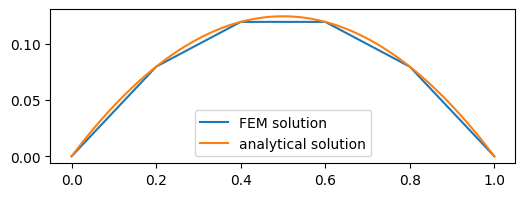
_images/e67562f9db2a84d19a3e17151ced432dcf8f56b860e29a1cdc94f128cd5bc9ec.png — Fig. 4 Solution of the boundary value problem using 1st order FEM#

Exercise

What is the system of equations if the trapezoidal rule is used to integrate the right-hand side?
Calculate the solution using the finite difference method and compare the two systems.
Why does the numerical solution in the nodes match the analytical solution exactly?

NGSolve solution#

Now let’s do the same with NGSolve

First, we create a one-dimensional mesh using netgen.

from netgen.meshing import Mesh as NGMesh # Caution: Mesh is also available in ngsolve!
from netgen.meshing import MeshPoint, Pnt, Element1D, Element0D
from ngsolve import *

m = NGMesh(dim=1)

# Number of subintervals
N = 5

# Points for the decomposition on the interval [0,1]
pnums = []
for i in range(0, N+1):
    pnums.append (m.Add (MeshPoint (Pnt(i/N, 0, 0))))

# Each 1D element (subinterval) can be assigned to a material.
# In our case, there is only one material.
idx = m.AddRegion("material", dim=1)
for i in range(0,N):
    m.Add (Element1D ([pnums[i],pnums[i+1]], index=idx))

# Left and right ends are boundary value points (0D elements)
idx_left = m.AddRegion("left", dim=0)
idx_right = m.AddRegion("right", dim=0)

m.Add (Element0D (pnums[0], index=idx_left))
m.Add (Element0D (pnums[N], index=idx_right))

# We have now defined the mesh
mesh = Mesh(m)

Now we create a \(H^1\) function space using this 1D mesh and the Dirichlet boundary points left and right.

V = H1(mesh,order = 1, dirichlet='left|right')
u = V.TrialFunction()
v = V.TestFunction()

# short cut
# u,v = V.TnT()

\(u,v\) are trial and test functions for the definition of the linear and bilinear function

a = BilinearForm(V)
a += grad(u)*grad(v)*dx

f = CoefficientFunction(1)
b = LinearForm(V)
b += f*v*dx

The two operators are now defined, but not yet calculated. The calculation is also called assembling. We will see later what this means in detail.

a.Assemble()
b.Assemble();

The matrix and the vector of the bilinear and linear form contain all degrees of freedom, in particular also the boundary points. However, these are given by the Dirichlet boundary values and do not need to be calculated (as mentioned above). We will take this into account when solving the system.

print(a.mat)

Row 0:   0: 5   1: -5
Row 1:   0: -5   1: 10   2: -5
Row 2:   1: -5   2: 10   3: -5
Row 3:   2: -5   3: 10   4: -5
Row 4:   3: -5   4: 10   5: -5
Row 5:   4: -5   5: 5

print(b.vec)

The GridFunction class is available in NGSolve for the solution itself. The trial and test functions are only used to define the problem and therefore have no memory for the solution vector, for example. The linear combination of the basis functions is automatically calculated in the evaluation of this. We need a GridFunction for the solution:

gfu = GridFunction(V)

Calculation of the FEM solution with NGSolve taking into account the free degrees of freedom:

gfu.vec.data = a.mat.Inverse(freedofs=V.FreeDofs())*b.vec

When the command is executed, the matrix is not inverted and multiplied to the vector from the left. That would be far too time-consuming numerically. Even if the notation claims otherwise, only the system of equations is solved.

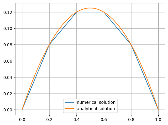
Again, we get the same result as above:

_images/5eb865fe3d40fbb2cafd832b4d7c7852930529517bacf4a8a74ee9d35bb15ebf.png

Extension into two-dimensional space#

Now let us look at the two-dimensional case. We will see that apart from the mesh, hence the region, the implementation in ngsolve remains identical. We consider the analog boundary value problem in two dimensions

\[\begin{split}\begin{split} -\Delta u & = 1 \quad\text{for}\ x\in \Omega\\ u & = 0 \quad\text{for}\ x\in \partial\Omega \end{split}\end{split}\]

on the unit square in \(\mathbb{R}^2\). For the weak equation follows

\[\int_\Omega \nabla u \cdot \nabla \varphi dV = \int_\Omega f(x) \varphi dV \quad \forall\ \varphi\in V \subset H_0^1(\Omega),\]

where \(V\) is a finite element space with \(\dim V < \infty\).

from ngsolve import *
from ngsolve.webgui import Draw

From netgen we import the unit square. With the help of the netgen module we can define and mesh 2d and 3d geometries.

from netgen.geom2d import unit_square

We now generate an unstructured mesh with a maximum edge length of 0.25:

mesh = Mesh(unit_square.GenerateMesh(maxh=0.25))

The size of the mesh can be controlled via the maxh parameter.

Draw(mesh);

What do the basis functions look like in two dimensions? To do this, we create an FEM function space and visualize the basis functions. The edge of the unit square consists of 4 lines, which have different labels:

mesh.GetBoundaries()

('bottom', 'right', 'top', 'left')

We define the H1 FEM function space with the Dirichlet boundary condition and initialize a GridFunction, an FEM function from the function space:

V = H1(mesh,order=1,dirichlet='bottom|right|top|left')
gfu = GridFunction(V)

Using the grid function, we can visualize the global basic functions. To do this, we set one coefficient to 1 and the others to 0. In the following example we visualize the 20th global basis function:

gfu.vec.FV()[:] = 0 # Initialize all entries with 0
gfu.vec.FV()[20] = 1

Draw(gfu,mesh,'u');

Using \(u(x) = \sum_i u_i\,\varphi_i(x) \in V\), as in the 1d example (4), the same system of equations follows

\[A(u,v) = f(v)\quad \forall \ v\in V,\]

with the bilinear form \(A: V \times V \to \mathbb{R}\)

\[\begin{split}\begin{split} A : V \times V & \to \mathbb{R}\\ (u,v) & \mapsto A(u,v) = \int_\Omega \nabla u\cdot \nabla v\, dV, \end{split}\end{split}\]

and linear form \(f: V \to \mathbb{R}\)

\[\begin{split}\begin{split} b : V & \to \mathbb{R}\\ v & \mapsto b(v) = \int_\Omega f(x)\cdot v\, dV. \end{split}\end{split}\]

For the definition in ngsolve we use again the proxy functions

u = V.TrialFunction()
v = V.TestFunction()

In two dimensions, we use dx to denote a surface integral and ds for a path integral (boundary integral). In our case we have for the bilinear form

A = BilinearForm(V)
A += grad(u) * grad(v)*dx

and analogously for the linear form

f = CoefficientFunction(1)
b = LinearForm(V)
b += f*v*dx

The right-hand side function onece again defined using a CoefficientFunction.

We have thus defined the bilinear form, which can be described in finite dimensions using a matrix, and the linear form, which can be described using a vector, but have not yet calculated them. The calculation of these is also called assembling.

A.Assemble()
b.Assemble();

The matrix \(A\) is in a sparse format stored. This means that only the matrix entries for which we potentially receive an entry are saved. The memory is not allocated at all for the rest of the matrix.

print(A.mat)

Row 0:   0: 1   4: -0.5   15: -0.5
Row 1:   1: 0.895075   6: -0.377531   7: -0.378808   18: -0.138736
Row 2:   2: 1   9: -0.5   10: -0.5
Row 3:   3: 1   12: -0.5   13: -0.5
Row 4:   0: -0.5   4: 1.92156   5: -0.31533   15: -0.15374   16: -0.95249
Row 5:   4: -0.31533   5: 1.8612   6: -0.198542   16: -0.307165   17: -1.04016
Row 6:   1: -0.377531   5: -0.198542   6: 1.79993   17: -0.395887   18: -0.827968
Row 7:   1: -0.378808   7: 1.84286   8: -0.324152   18: -0.918526   19: -0.22137
Row 8:   7: -0.324152   8: 1.79252   9: -0.271716   19: -0.860521   20: -0.336129
Row 9:   2: -0.5   8: -0.271716   9: 2.02128   10: -0.0759864   20: -1.17357
Row 10:   2: -0.5   9: -0.0759864   10: 1.81976   11: -0.220817   20: -0.288822   21: -0.734131
Row 11:   10: -0.220817   11: 1.84084   12: -0.448101   21: -0.875576   22: -0.296345
Row 12:   3: -0.5   11: -0.448101   12: 1.87   13: -0.26789   22: -0.654007
Row 13:   3: -0.5   12: -0.26789   13: 1.84321   14: -0.506823   22: -0.367252   23: -0.201248
Row 14:   13: -0.506823   14: 2.01367   15: -0.420679   23: -1.08617
Row 15:   0: -0.5   4: -0.15374   14: -0.420679   15: 1.79625   16: -0.418051   23: -0.303778
Row 16:   4: -0.95249   5: -0.307165   15: -0.418051   16: 3.61084   17: -0.609253   23: -0.717205   24: -0.606678
Row 17:   5: -1.04016   6: -0.395887   16: -0.609253   17: 3.78711   18: -0.965502   24: -0.77631
Row 18:   1: -0.138736   6: -0.827968   7: -0.918526   17: -0.965502   18: 3.86126   19: -0.936881   24: -0.073651
Row 19:   7: -0.22137   8: -0.860521   18: -0.936881   19: 3.63019   20: -0.534253   24: -0.503238   25: -0.573927
Row 20:   8: -0.336129   9: -1.17357   10: -0.288822   19: -0.534253   20: 3.74798   21: -0.678509   25: -0.73669
Row 21:   10: -0.734131   11: -0.875576   20: -0.678509   21: 3.72565   22: -0.616041   25: -0.821391
Row 22:   11: -0.296345   12: -0.654007   13: -0.367252   21: -0.616041   22: 3.58077   23: -0.913832   24: -0.139859   25: -0.593436
Row 23:   13: -0.201248   14: -1.08617   15: -0.303778   16: -0.717205   22: -0.913832   23: 3.76762   24: -0.545392
Row 24:   16: -0.606678   17: -0.77631   18: -0.073651   19: -0.503238   22: -0.139859   23: -0.545392   24: 3.67338   25: -1.02825
Row 25:   19: -0.573927   20: -0.73669   21: -0.821391   22: -0.593436   24: -1.02825   25: 3.7537

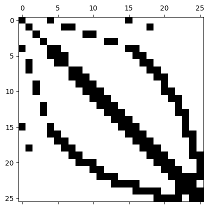
We can also regard this matrix (at least as long as it is small!) as a dense matrix:

rows,cols,vals = A.mat.COO()

denseA = np.zeros((np.max(rows)+1,np.max(rows)+1))
k=0
for i,j in zip(rows,cols):
    denseA[i,j] = vals[k]
    k+=1

plt.spy(denseA)
plt.show()

_images/e6866bd022189b86a22e9a99a5b201498a942d9e28fbd46f0653b07815f1452f.png

We can also use scipy.sparse for further computations.

import scipy.sparse as sp
Asparse = sp.coo_matrix((vals,(rows,cols)))
plt.spy(Asparse)

<matplotlib.lines.Line2D at 0x10ee2f250>

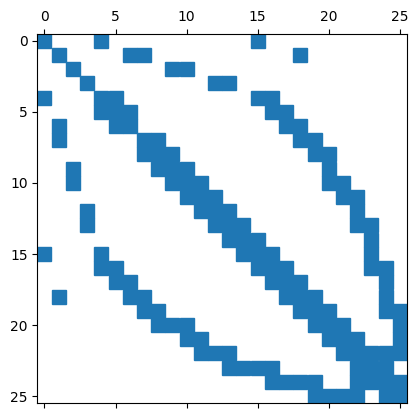
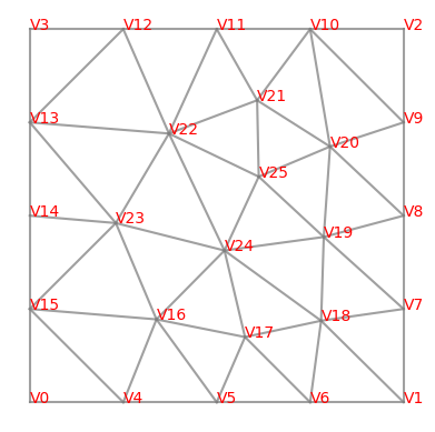
_images/a087943f5bc1333339e2d543a3c7a4c67bae1e014565d73fae1114a96a2abf6a.png

The pattern of the matrix entries depends on the numbering of the nodes (from the meshing) and the FEM basic functions. It is also possible to draw the mesh directly with matplotlib; the mesh object contains all the information required for this.

for e in mesh.edges:
    line = np.array([mesh.vertices[v.nr].point for v in e.vertices])
    plt.plot(line[:,0],line[:,1],c='gray',alpha=0.75)
for v in mesh.vertices:
    plt.text(*v.point,v,color='red')
plt.gca().set_axis_off()
plt.gca().set_aspect(1)
plt.show()

_images/e2722305ad9303f7d23996126d664a86f119eeaa56c08255376555c0feb1a7be.png

We now consider the free degrees of freedom, for which we must keep the homogeneous Dirichlet boundary condition in mind. The number of free dof’s is given by

freedofs = V.FreeDofs()
print(freedofs)
freedofsnp = np.array([i for i in freedofs])

0: 00000000000000001111111111

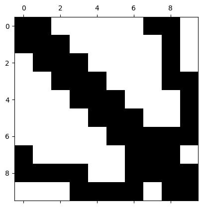
As we can see, the order of numbering the nodes is via the corners, edges into the interior. Thus, the degrees of freedom available to us are at the end. The matrix pattern for solving the problem is given by

ind = np.arange(freedofsnp.shape[0])[freedofsnp]
plt.spy(denseA[np.ix_(ind,ind)])
plt.show()

_images/e969ca2575f4c792b9007b4693d6a933061a1c54ec1f0cf82b49fda29250e8e2.png

Let’s solve the system for the inner degrees of freedom:

gfu.vec.data = A.mat.Inverse(freedofs=V.FreeDofs())*b.vec

Draw(gfu,mesh,'u');